Why Quantile Regression?

One of the projects we are working on is predicting the future positions of agents based on past observations. As we all konw such prediction cannot be accurate when it goes far to the future. The question is then, how inaccurate?

Techniques such as VAE can be used to regress the target value as well as the distribution, which gives you some idea about how uncertain the value is. However, VAEs are hard to train and therefore less practical.

One of my colleagues introduces us the quantile regression as an alternative. Quantile regression does not directly estimate the distribution. Instead, it answers questions such as:

• What is the mean (50% percentile) of the distribution?
• What is the 80% percentile of the distribution?

Such estimation is not as precise as the distribution since it only estimates some statistics about the distribution. However, in practice it is usually good enough and even more useful to do so since that is how you are going to use the distribution anyway.

What is Quantile Regression?

The key of quantile regression as I understand it is about a series of slightly tweaked loss functions. I found the inutition behind them very interesting, and decieded to write about them to help others better understand them.

The most widely used loss function used in supervised learning (e.g. the regression we are talking about) is mean square. Mean square loss can be written as the sum (actually mean, but the quantity is a constant anyway) of $f_i(y) = (y - y_i)^2$.

Let’s first try to reason about the mean square loss, i.e. how does it drive the optimization (training). Imagine you choose some parametrized function to estimate $y$, for example a neural network, and use mean square loss as the last layer. If we look at how the backward pass of the last layer alone guide the optimization, it is striaght forward to see that it is trying to get $y$ to its optimal value, which is the mean of all the $y_i$.

Quantile losses are not so different from the ordinary mean square loss. In fact, they are just replacing the $f_i(y)$ with L1 norm and its friends (in mean square loss, it is L2 norm).

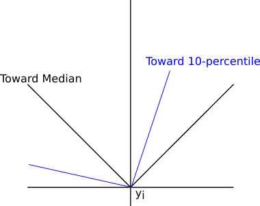
In the above graph, there are two examples of quantile losses.

1. $f_i(y) = |y-y_i|$, which guides the value toward the median (50-th percentile) of $y_i$
2. $f_i(y) = \begin{cases}0.1 * |y_i - y| & y < y_i\\0.9*|y - y_i| & y \geq y_i\end{cases}$, which guides the value toward the 10-th percentile of $y_i$.

It might be hard to grasp how quatile losses can do that at the first glance. It actually follows quite simple intuitions.

Intuition behind the Quantile Losses

Let’s first look at the L1 loss, which is dicated in the previous section to drive $y$ toward the median. Similar to how we did the analysis for the mean square loss, we ask ourselves one question: without any constraints, what is the optimal $y$ that minimizes the loss? Note that this is equivalent to analyzing the (partial) effect of the backward pass of the last layer, if L1 is used as the loss.

Assuming there are in total 101 different $y_i$, and $y’$ is an arbitrary value. If there are 30 $y_i$ on the left of $y’$ and 71 on the right, what is the derivative of the sum of $f_i$ at $y’$. Well if we move $y’$ slightly to the right by the amount of $h > 0$ at $y’ + h$, it is quite easy to figure out that the shift in the sum of $f_i$ would be $30h - 71h = -41h$ if $h$ is small enough. The derivative is then $-41$ by definition. This means that we keep moving $y’$ to the right, the loss drops. I think by now it is clear that the derivative is always going to be negative as we move $y’$ to the right, until it reaches the median! Therefore, we figured out how this loss drives $y$ toward the median.

The anlysis of an arbitary quantile losses $f_i$ then follows immediately.

$$ f_i(y) = \begin{cases} p * (y_i - y) & y < y_i \\ (1 - p) * (y - y_i) & y \geq y_i \end{cases} $$

Still, doing the same imaginary experiment with an arbitrary $y’$ moving along the axis. In this case, we penalize differently for $y_i$ on the left side and right side. If we have $q%$ on the left side and $(100 - q)%$on right side, the spot derivative is proportional to $q% * (1 - p) - (100 - q)% * p$. It is easy to see the derivative monotonically increases (or decreases) to 0 when $q% = p$. This means that $y$ minimizes the sum of such quantile loss at $p$ percentile!

Use of Quantile Losses

There are many articles talking about how to make use of such quantile losses. And they are indeed useful. 90% and 10% percetile estimation already tell you enough about how uncertain your estimation is.

Read this post for more about the applications.